
| Markov-Based Reconstruction Mechanism |  |
Windographer's Markov-based reconstruction mechanism generates artificial data to fill gaps in a measured time series. The artificial data matches the measured data in terms of frequency distribution, seasonal and diurnal patterns, and autocorrelation. This article describes the four steps of this process, shows several examples of its output, and discusses its limitations.
In the first step of the process, Windographer analyzes the diurnal and seasonal patterns of the measured data as it generates its seasonality profile. For every day of the year and for every time step of the day, it assembles a distribution of observed values, so that for each time step of the year it has a record of the lowest value, the highest value, the 10th, 20th, 30th percentile values, and so on, observed for that time step.
The graph below, for example, shows a portion of the results of such an analysis. Of the values observed in the time step 12:00pm - 12:10 on May 23, the 10th percentile was about 9°C, the 20th percentile was about 12°C, the 30th percentile was about 13°C, the 70th percentile was about 16°C, the 80th percentile was about 17°C, and so on. The distribution of values varies from one time step to the next, and from one day to the next, as a result of the diurnal and seasonal patterns in the observed data.
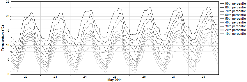
In generating the seasonality profile, Windographer uses a moving window that incorporates more than just the time step at the center of the window, and more than just the day at the center of the window. The article on the seasonality profile explains.
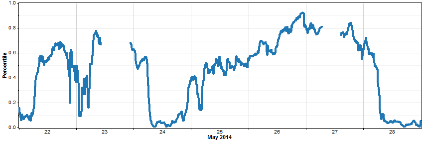
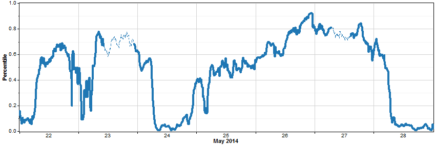
In the second step of the process, Windographer removes the seasonality profile (as described in the article on seasonality profile) to create the 'seasonality-normalized time series'. To see how to construct such a time series, let's look again at the temperature data we saw in step 1. The graph below shows the same percentile data that we saw above, for the same seven days of May, but this time the observed temperature for May 2014 appears as well. The graph shows that early on May 24, 2014, the temperature was quite low relative to all the values observed for that day of the year and that time of day -- it was about as chilly as it gets for early on May 24. But over the next 48 hours the percentile value of the temperature rose fairly steadily, so that by late on May 26, 2014, the temperature had reached the 90th percentile -- about as warm as it gets for late in the day on May 26.
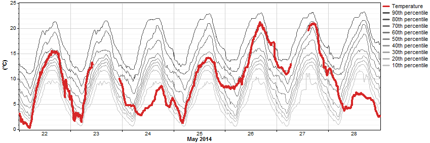
For any temperature value that appears in the graph above, we can calculate the corresponding percentile value. The resulting 'seasonality-normalized time series' would look like this:
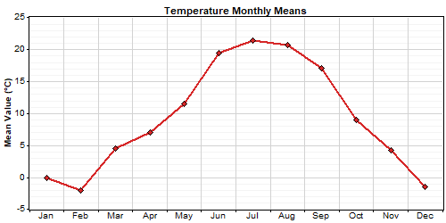
Removing seasonal and diurnal patterns simplifies the properties of the time series significantly. The original temperature time series shown above, for example, has the following seasonal profile, diurnal profile, and frequency histogram:
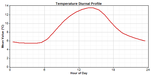
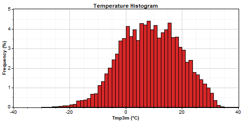
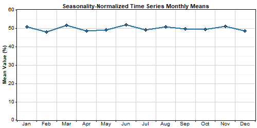
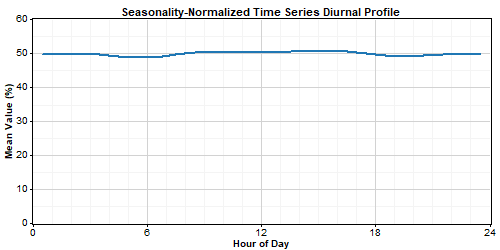
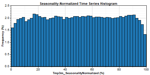
After removing the seasonality profile, the resulting seasonality-normalized time series exhibits virtually no seasonal pattern or diurnal pattern, and has a nearly uniform frequency distribution:
In the third step of the process, Windographer fills the gaps in the seasonality-normalized time series. It does so by constructing a Markov transition matrix, then generating random numbers to construct from the transition matrix an artificial scenario to fill each gap. If the last synthetic value (at the end of the gap) matches poorly with the first measured value after the gap, Windographer discards that scenario and constructs another until it finds one that closely matches the measured data at both ends of the gap.
The graph below shows the same seasonality-normalized time series we saw above, this time with the gap fills appearing as thin dotted lines:
When filling gaps, we intend to generate artificial data segments that closely match the statistical properties of the real data. By first removing the seasonality profile, and then filling gaps in the seasonality-normalized time series, we have greatly improved our chances of achieving this match. That's because whereas the original time series exhibits seasonal and diurnal patterns, and has an arbitrary frequency distribution, the seasonality-normalized time series displays no seasonality at all, and it has a uniform distribution. It usually exhibits autocorrelation, meaning a tendency for the value in one time step to depend somewhat on the value in the previous time step, but the Markov transition matrix captures this property very well.
In other words, we have simplified the time series to a point where we can successfully synthesize data segments that behave just like it. Having filled all gaps in this way, we are ready for the next step of the process.
In the fourth and final step of the process, Windographer converts the seasonality-normalized time series back to physical units by factoring back in the seasonality profile. The article on seasonality profile describes this process in detail, but we can see it at work in our sample time series.
Near noon on May 23, 2014, for example, we synthesized a percentile value of about 0.7. The graph at the top of this page shows that the 70th percentile value for noon on May 23 is about 16°C, so our synthesized temperature value for that time step is roughly 16°C. Doing this for all synthesized percentile values gives the following graph, with the gap fills again appearing as thin dotted lines:
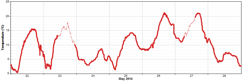
Note how the diurnal pattern re-emerges in this final step. For example, although we generated a roughly flat section of synthetic percentile values to fill the gap in the seasonality-normalized time series on May 23, 2014, the corresponding synthetic temperature values display the diurnal profile characteristic of that time of year.
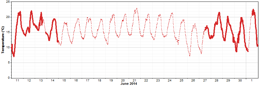
Even much longer gap fills faithfully replicate the appropriate diurnal and seasonal patterns. The graph below, for example, shows the same temperature dataset over a three-week period of June 2014, much of which was originally missing. The gap fill scenario may not reflect what actually happened during that nearly two-week gap, but it does reflect a realistic diurnal pattern and a realistic amount of random deviation from one time step to the next.
The following time series graphs show the results of the Markov-based reconstruction mechanism working on wind speed data. In these cases the algorithm has produced synthetic wind speed data quite different in character from the synthetic temperature data we saw above, but as in the cases above, the synthetic data closely mimics the behavior of the original data.


A closer look at the properties of the synthesized wind speed data shows that, as we would expect, the synthetic data matches the real data in terms of seasonal pattern, diurnal pattern, and distribution:
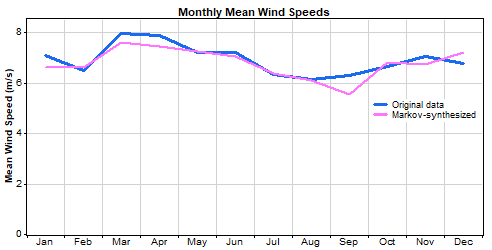
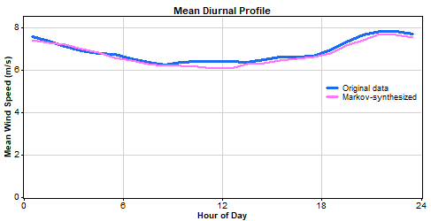
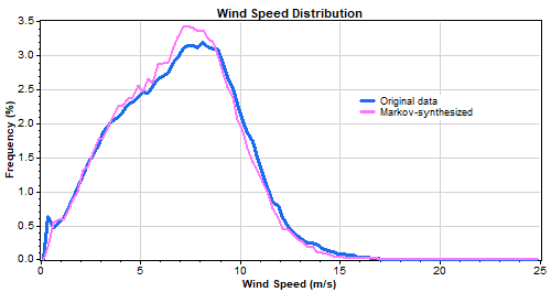
The graphs above show that the Markov-synthesized data matches the real data in terms of overall statistics. But at the time series level, how well does Markov-synthesized data compare to real data? To test this, we deleted segments of real 10-minute wind speed data, reconstructed them with the Markov mechanism, and then plotted the original and synthetic data on the same graph.
Short 6-hour synthetic segments followed the real segments fairly well, partly because the Markov mechanism ensures that the synthetic segment matches the real data at its start and end, and the short intervening interval limits the creativity of the mechanism:

By chance, some synthetic segments match the real behavior very well, as in the leftmost example below, but more often they follow a somewhat different path:

With longer 24-hour gaps, the Markov-synthesized segments will more likely deviate substantially from the actual data, since 24 hours is long enough to allow many different possible paths, and there is no guarantee that the Markov mechanism will synthesize the one path that actually occurred. In some cases it gets quite close:

But in others it synthesizes quite a different path:


And occasionally it synthesizes a virtually opposite path, as in the following example where the synthetic segment goes up and then down, even though the real data segment went down and then up:

This method of appraising the 'accuracy' of a Markov gap fill becomes less and less legitimate as the length of the segment increases. The purpose of the Markov mechanism is to produce statistically defendable artificial data in times that lack not only primary data but even secondary data that we could use as a reference. (The pattern-based and MCP-based reconstruction mechanisms exist to fill gaps during times of valid reference data.) So Windographer deploys the Markov mechanism only when it has absolutely no indication of what actually happened. We would therefore expect that the Markov mechanism could sometimes synthesize a segment that happens to take a very different path than the real data. But even such a segment as that must be considered successful if the synthetic segment exhibits statistically realistic behavior appropriate to the season and time of day, and if it matches up well with the real data at the start and end of the gap.
The most important limitation of this reconstruction mechanism is that it does not depend on any concurrent reference data, which is to say that it knows nothing about what actually happened in the missing segments. This distinguishes it from the other reconstruction mechanisms, which refer to concurrent data from other datasets or other sensors in the same dataset to give some indication of what happened in the missing segment. The Markov-based mechanism does not do that, but rather simply aims to fill gaps with artificial data that behaves just like the real data. It therefore risks producing a synthetic segment very different from what actually happened, because even if an artificial data segment displays perfectly realistic statistical properties, it may still diverge strongly from the actual data segment. In other words, as in the example we just saw, the Markov mechanism might synthesize a segment that perfectly matches the real data's statistical properties, but goes up and then down whereas the real segment went down and then up.
Even the mechanism's ability to match the real data's statistical properties has its limits. At the end of our explanation of step 3 of this process, we stated that the statistical simplicity of the seasonality-normalized time series allows us to synthesize artificial data segments that behave just like it. Strictly speaking, that may not be true. It tends to be true for most meteorological variables like speed and temperature, whose seasonal and diurnal patterns typically account for almost all of the statistical complexity of the time series. In such cases, removing seasonality really does yield a time series with very simple statistical properties, and the Markov transition matrix captures those remaining properties very well.
However, other factors can also drive the behavior of a time series. Electrical load data, as an example, tends to exhibit not just seasonal and diurnal patterns, but also strong weekly patterns because we tend to consume electricity differently on weekends compared to weekdays. Windographer's Markov-based reconstruction mechanism would not account for this weekly pattern because it does not consider the day of the week in its normalization process. It should synthesize April data that looks like real April data, and November data that looks like real November data, but it would not distinguish between a Sunday in April and a Monday in April. A demonstration appears in the next section of this article.
Similarly, the Markov-based reconstruction mechanism does not account for seasonal changes in Markov transition probabilities. For example, if in a particular location the temperature tended to exhibit strong autocorrelation in the summer but weak autocorrelation in the winter because of frequent storm fronts, then Windographer's use of a single Markov transition matrix for the entire year would cause it to synthesize insufficiently-autocorrelated data in the summer and overly-autocorrelated data in the winter.
A diurnal or directional dependence of the Markov transition probabilities would lead to a similar oversimplification. The process also ignores long-term trends in the data, so it synthesizes data without regard to any such trends.
Despite these limitations, the Markov-based reconstruction mechanism performs well on a wide variety of data types that, like speed or temperature, are driven by seasonal and diurnal forcing, or that are in turn driven by such meteorological variables.
Electric load data tends to exhibit seasonal and diurnal trends, but as mentioned above it also tends to exhibit a significant weekly trend because people tend to use eletricity differently on weekends than on weekdays. Because Windographer's Markov-based reconstruction mechanism ignores the day of the week, we do not expect it to reflect any weekly pattern in its output. To test that hypothesis, we will create and fill a gap in an electric load dataset showing the total Alberta electrical system demand. The graph below shows a five-week sample of that data, highlights weekends, and indicates the three-week segment of data that we deleted to perform this test.

The graph below shows the three-week segment generated by Windographer's Markov-based reconstruction mechanism.

The above graph confirms that, as we expected, the synthesized data fails to replicate the observed weekly pattern. It replicates the observed diurnal pattern respectably well, and it even produces a realistic mixture of high-demand and low-demand days, but those days do not follow the observed weekly pattern.
Electric load data is driven partly by meteorological variables and partly by human behavior, and as described above, Windographer's Markov-based reconstruction mechanism accounts well for the seasonality in meteorological variables, but does not account for weekly patterns or any other type of pattern.
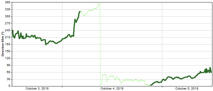
Windographer treats wind direction data in a special way because of its vector nature. To fill gaps in a wind direction data column, Windographer begins by calculating the vector wind velocity in each time step, using the associated wind speed sensor for the magnitudes of the vectors. (If the direction sensor has no associated speed sensor, it assumes unit vectors, meaning that each vector has the same magnitude). It then converts these vectors into scalar N-S speeds and E-W speeds, fills the gaps in the N-S speed and E-W speed data columns, then converts back to vector wind speeds and sets the missing direction values equal to the directions of the vectors. (It does not use the vector magnitudes.)
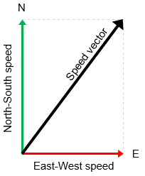
An example of the result of this approach appears below. In this case, the synthetic direction data that Windographer generates to fill the gap make a realistic transition from a NNW (near 330°) to NNE (near 5°), passing through due north on its way. Had Windographer treated the wind direction as a scalar variable, that transition would have likely taken more of a straight-line trajectory that would have instead passed through due south.
The Markov algorithm does not try to make the average or the values that it inserts into the time series match the values in the rest of the time series. Nor does it scale the final time series so that its final average value matches its average before the insertion of synthetic data. As a result, it can change the mean value of the time series.
But the Markov process works on the seasonality-normalized time series, defined above. The seasonality-normalized time series consists of percentile values, each one indicating the value in a particular time step relative to all the observations of valid data made in nearby time steps, meaning nearby days of the year and nearby hours of the day. Once Windographer re-applies the seasonality profile in step 4 of the process, the resulting synthesized values are guaranteed not only to fall within the range of the true values observed in similar time steps, but also to match the distribution of values observed in similar time steps.
In other words, the values that the Markov algorithm inserts are drawn randomly from the distribution of observed values. They are drawn very carefully from that distribution so as to match the real seasonal and diurnal patterns and autocorrelation behavior, but ultimately they are drawn from the distribution of observed values. That means the Markov algorithm will not distort the average of the time series. That’s not the same as saying the average value won’t change, but it’s actually much better.
If you are filling gaps in a temperature time series, for example, and you have lots of summer and winter data showing that it’s warm in the summer and cold in the winter, and you have many more gaps in the winter, then the simple mean of the observed data will be too high because it will be seasonally biased towards the summer – it’s based on more summer data than winter data. In that case the perfect gap fill process will reduce the mean temperature because it will insert realistic (cold) winter temperatures in the winter and realistic (warm) summer temperatures in the summer, but it will insert more winter data than summer data because most of the gaps occur in the winter. The Markov algorithm will do exactly that. Similarly, if mornings differ from afternoons in the observed data, and if the Markov algorithm inserts more morning data than afternoon data, then it will change the character of the data, but in an appropriate way, to remove the bias in the observed data.
The Markov-based reconstruction mechanism forms part of the process of reconstruction within a data set, which happens in the Reconstruct Single Dataset window of Windographer. It also figures in the Matrix Time Series MCP algorithm.
See also
Pattern-based reconstruction mechanism
MCP-based reconstruction mechanism
Process of reconstruction within a dataset