
| Matrix Time Series MCP Algorithm | |
The 'Matrix Time Series' (MTS) algorithm (Lambert and Grue, 2012) is an adaptation of the classic matrix method (Anderson and Bass, 2004), modified to produce realistic time series data.
The MTS algorithm, like the classic matrix method, aims to generate a realistic distribution of wind speeds at the target site. This attention to the target speed distribution is the main advantage of the matrix-based algorithms over most linear MCP algorithms, which tend to generate an unrealistic distribution at least part of the time.
Part of the MTS method’s approach to generating a realistic target distribution is to recognize the probabilistic nature of the relationship between target and reference wind speeds: a single reference speed will correspond not to a single target speed, but rather to a distribution of target speeds. For example, if you were to look at the concurrent measurement period and focus on the time steps in which the reference speed is near, say, 10 m/s, you might find that the target speeds in those time steps will sometimes be 15 m/s, sometimes 12 m/s, sometimes 7 m/s. The joint probability distribution, which describes this probabilistic relationship, is at the heart of the MTS algorithm.
The MTS algorithm comprises the following steps:
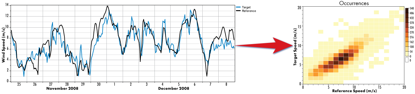
The fundamental idea behind matrix-based MCP methods is to use the complete 2-dimensional joint probability distribution of the target and reference wind speeds to generate the predicted wind speed data. Not only does this allow the algorithm to model arbitrary nonlinear relationships between the target and reference site, it also preserves information about the variance in each variable (as opposed to, for example, basic linear regression, which maps a single specific target wind speed to every given reference wind speed value). Therefore the first step of the MCP method is to build this joint probability distribution (JPD).
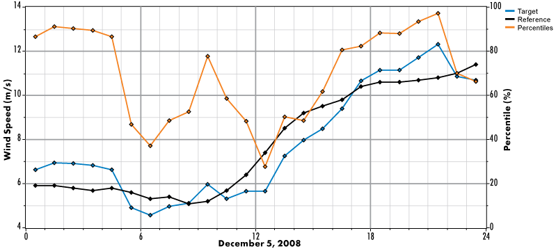
The next product of the MTS algorithm is the 'percentile time series'. This is another set of time series data points that Windographer generates as an intermediate output of the MTS algorithm. In each time step, Windographer takes the concurrent target and reference wind speeds, chooses from the JPD the column corresponding to the appropriate reference speed bin, and from that constructs the CDF of target wind speeds observed in that bin. Finally, from this CDF Windographer calculates the percentile value corresponding to the observed target wind speed. To see the percentile time series, click the Percentiles graph radio button.
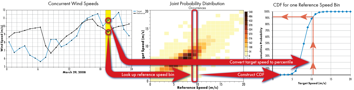
A simple way to think of the percentile time series is that each percentile value represents how windy the target site is compared to how windy we would expect it to be, given the current reference wind speed. Therefore a percentile value of 0.5 or 50% means that, in this time step, the target wind speed is exactly the average of what we would expect, given the reference wind speed in that time step. In the same way, percentile value of 90% would indicate an unusually windy target site, a value of 10% would indicate an unusually calm target site, etc. Because the distribution of target wind speeds will vary depending on the range of reference wind speeds considered, the same value of the percentile time series can of course represent different target site wind speeds in different time steps.
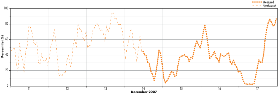
In this step, Windographer uses the Markov-based reconstruction mechanism to fill gaps in the percentile time series. The synthesized data respects the seasonal and diurnal patterns in the original percentile time series, as well as the characteristic autocorrelation, and matches up with the 'edges' of any gaps in the original target site data.
The final step is for Windographer to transform the synthetic percentile time series values into synthetic target wind speed values. Windographer does this by referring back to the JPD and using it to calculate the expected target wind speed value for the given percentile value and reference wind speed in each time step, essentially reversing the 'Build the Percentile Time Series' step. Once again Windographer calculates the CDF of target wind speed values for the given reference wind speed, only this time it uses the percentile value to look up the predicted target wind speed value for that time step. Whereas the previous step was concerned with preserving the seasonal and diurnal patterns and autocorrelation of the data, it is really this step that is concerned with preserving the statistical relationship between target and reference wind speeds, as it does by consulting the JPD.
![]()
The Matrix Time Series algorithm supports the following options:
The Direction sectors drop-down box allows you to subdivide the data by direction sector, as defined by the reference direction sensor. Windographer calculates a separate JPD for each direction sector, and then when it creates the percentile time series, in each time step it refers to the appropriate JPD according to the reference direction in that time step. It still puts all of the percentile values into the same percentile time series though, and directional subdivision has no effect on step 3 of the algorithm. Then in the final step, when transforming the percentile values back into target wind speeds, it again refers to the appropriate JPD for each time step, depending on the reference direction in that time step.
Reference speed bin size and Target speed bin size refer to the sizes of the bins used to produce the JPD. Smaller bins will produce a more fine-grained JPD, but if the bins are too small then the JPD will begin to suffer from sparsity problems (i.e. some bins will have little or no data). The MTS method does use a backup method when sparsity begins to occur however: when the total number of data points for a given reference wind speed bin is less than 10, Windographer will fall back to predicting the target wind speed based on a simple least-squares curve fit for the appropriate direction sector. It must be stressed that this is just a backup so that Windographer doesn't have to synthesize gaps in case of sparse data. In the worst case where most bins are sparse, the performance of the MTS method will tend towards that of the LLS method. Therefore sparsity should be avoided by making the bin sizes large enough.
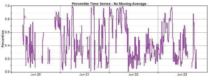
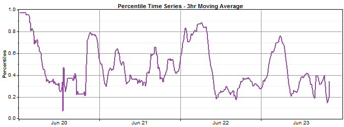
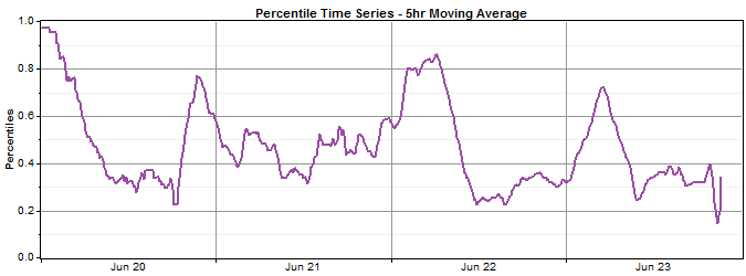
The Moving average window controls the size of the moving average used when calculating the percentile time series. Because the percentile values are calculated based on a CDF of target wind speeds (as explained above), the percentile values can sometimes vary erratically, especially at high and low values where data is scarce. Therefore Windographer offers the ability to smooth the percentile time series by calculating a moving average. For example, if the time step is 60 minutes and the moving average window is set to 3 hours, each percentile value will really represent the average of 3 percentile values (one central time step and one on either side). The graphs below show the effect of increasing the moving average window on the smoothness of the percentile time series (in order, no moving average, 3 hours, 5 hours).
See also
Markov-based reconstruction mechanism