| Simple Algorithm for Gumbel Fitting |  |
The Simple algorithm for fitting the Gumbel distribution does a straightforward linear least squares fit to find the two parameters of the Gumbel distribution. The basis of this algorithm is the equation for the cumulative distribution function of the Gumbel distribution:

Taking the logarithm of both sides twice and rearranging leads to the following equation:

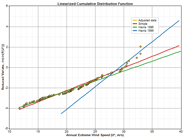
That is in the form y = mx + b, so if we plot -ln(-ln(F(x))) versus x, we get a straight line with a slope of 1/b and an intercept of -m/b. The Simple algorithm for Gumbel fitting performs this process.
The graph below shows 92 monthly peak wind speeds along with the Gumbel distribution resulting from the Simple algorithm and two more sophisticated Gumbel fit algorithms, the Harris 1996 algorithm and the Harris 1999 algorithm:

You can apply the Simple algorithm on the Extreme Wind Tool window, but not the Extreme Wind window.
The Simple Gumbel fit algorithm uses the same orientation of the axes that Harris suggested Harris, 1996, in which the observed wind speeds appear on the x-axis and the probabilities on the y-axis. The linear least squares regression algorithm This arrangement recognizes that the true uncertainty lies in the probability values rather than the measured wind speeds.
See also