
| Larsen & Hansen Turbulence Detrending Algorithm | |
In Windographer documentation, the 'Larsen & Hansen Turbulence Detrending Algorithm' refers to the algorithm put forward in section 4.1 of Larsen and Hansen (2014), which is the on-shore variant of what that paper calls Method 2.
The physical loads on a wind turbine depend strongly on the turbulence intensity, so wind energy modelers strive to determine accurately the turbulence conditions to which turbines will be exposed. But the fact that the wind industry tends to record wind resource data on 10-minute intervals makes this determination more difficult.
Of particular importance to fatigue loads in the turbines are the high-frequency (on the order of 1Hz) fluctuations in the wind. Historically the wind industry has assumed that the quantity of such high-frequency fluctuations is well approximated by the raw turbulence intensity, defined as the ratio of the standard deviation of measurements made with the 10-minute time step to the mean of those measurements. That assumption is accurate in the absence of a trend in the wind speed over that 10-minute time step. But if the wind is trending strongly up or down over that time step, then the standard deviation over the time step will result partly from that trend and partly from the high-frequency fluctuations superimposed over the trend. The point of turbulence detrending is to subtract the contribution of the longer-term trend and thereby calculate more accurately the quantity of high-frequency fluctuations within each 10-minute time step.
The Larsen and Hansen paper puts forward two approaches, which they call models, to calculate detrended turbulence intensity time series from typical 10-minute wind resource data. Both approaches analyze each time step by focusing on a 30-minute window of time comprising the time step of interest at the center, flanked by the time steps before and after. Both approaches fit a third-order polynomial curve to the measured data to serve as a hypothetical trendline over the 30-minute period, then calculate for the time step of interest the standard deviation that would result purely from that trendline, in the absence of any high-frequency fluctuations, and finally subtract that from the measured standard deviation to find the standard deviation assumed to result purely from high-frequency fluctuations.
The two approaches differ in how they fit the polynomial trendline over each 30-minute period. The first approach, which the authors call Method 1, makes use only of the three measured mean wind speeds in the three time steps in the 30-minute window. The second approach, which they call Method 2, makes use of the three measured standard deviations values as well. The paper concludes that Method 2 leads to "a significantly more precise estimate of the trend contribution" to the measured standard deviation. Windographer implements Method 2.
The Larsen and Hansen paper further subdivides Method 2 into two variants, one for onshore conditions in which the surface roughness is constant, and one for offshore conditions in which the surface roughness varies with the mean wind speed, since higher wind speeds tend to cause higher waves. Windographer implements the onshore variant of Method 2.
Please refer to Larsen and Hansen (2014) for a detailed description of the algorithm.
To apply the Larsen and Hansen detrending algorithm to any turbulence intensity data column, go to the Configure Dataset window, double click on the TI column to see its properties, and check the checkbox to apply the detrending algorithm:
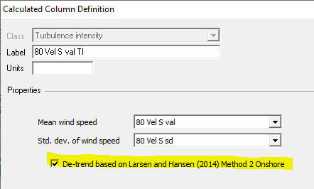
Whether or not you apply the Larsen and Hansen algorithm to your TI columns in this way, you can explore the implementation and effects of the Larsen and Hansen algorithm in the Turbulence Detrending window.
See also
Turbulence intensity calculated column