
HOMER Pro 3.16

The Modified Kinetic Model (or ASM) is based on the Kinetic Battery Model (Manwell and McGowan, 1993). The Modified Kinetic Model adds a series resistance, temperature effects on capacity, temperature effects on degradation rate, and cycle-by-cycle degradation based on depth of discharge (DOD). The model uses commonly available data (some battery datasheets, for example, provide all the necessary information to define the complete model), and is designed so that parts of the model can be left out if data is not available, the model is not representative of the real behavior, or the behavior does not apply for the conditions being modeled.
Tip: Be sure to specify weight when creating a Component with the Modified Kinetic Battery Model. The model uses the weight to calculate heat transfer and thermal behavior.
The different aspects of the model combine linearly and are easy to isolate so the data entered to generate the model can be reproduced in simulation. For example, you can enter a lifetime versus temperature curve that includes a point at 40°C and five years. You can create a model with the temperature fixed at 40°C and the battery not used (so cycle life is not a factor). You can check that the battery is replaced every five years. Basically, the model is as simple as possible while still including all of the desired phenomena.
See the Kinetic Battery Model section of the help for a review of the Kinetic Battery Model (KiBaM) and the maximum capacity, capacity ratio, and rate constant parameters. This section explains the details and function of the Modified Kinetic Model. For information about defining a Modified Kinetic Battery in the library, see the Modified Kinetic Battery Model section of the help.
Functional Model
The time-step-to-time-step behavior of the battery in simulation is governed by the functional model.
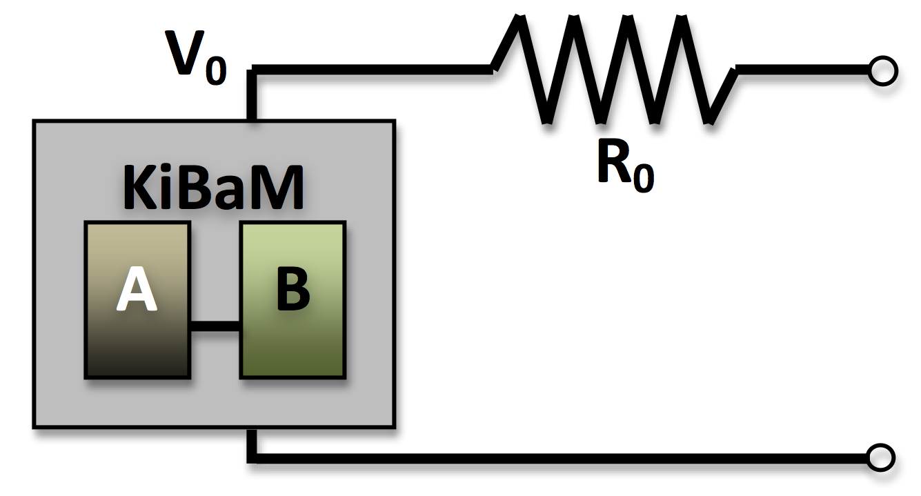
For a given power output, the current, I, is defined as:
Pout = IVoutput = V0I - R0I2 (1)
This quadratic equation is solved for the current, I. This current is then applied to the Kinetic Battery Model to determine the state for the following time step. The equations used for this are described in the Kinetic Battery Model section of the help.
The maximum discharge power and maximum charge power are calculated similarly to the regular Kinetic Battery Model. In addition, there is a maximum discharge power limit imposed by the circuit model, which is found by determining which current gives the maximum value of Pout for the quadratic function in (1):
IPout,max = V0 / (2 R0) (2)
Thermal Model
The Storage Component temperature is modeled as a lumped thermal capacity. You specify the thermal conductance to ambient (watts per kelvin), the mass of the component (pounds; multiply kilograms by 2.20 to convert to pounds), and the specific heat capacity (joules per kilogram-kelvin). If you specify a specific heat capacity of zero, the battery internal temperature follows the temperature resource exactly.
Tip: If you do not select "Consider temperature effects?" in the site-specific inputs of the Storage page, the battery internal temperature stays constant at the temperature specified in the Library. In this case, the thermal model is not used.
In each time step of the simulation, any energy dissipated by the effective series resistance is converted to heat and increases the bulk temperature of the storage bank. Additionally, heat dissipates to or is absorbed from the surroundings according to the convection equation: q = hΔT. You can specify the ambient temperature for simulation in the temperature resource. Losses specified by the "Other round-trip losses" input are not converted to heat in the thermal model.
Losses in the series resistance are converted to heat:
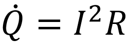
where I is the current in amps, and R is the series resistance in ohms.
The rate of change of the battery's internal temperature is driven by this heat generation and the rate of heat exchange with ambient. This can be described as an energy balance:
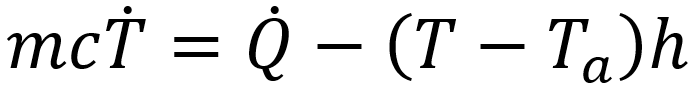
where: |
|
|
|
m |
= the mass of the battery [kg] |
|
c |
= the specific heat capacity [J/kgK] |
|
h |
= the thermal conductance to ambient |
|
T |
= [Kelvin, with rate of change in Kelvins per second] |
|
T |
= the internal temperature of the battery |
|
Ta |
= the ambient temperature |
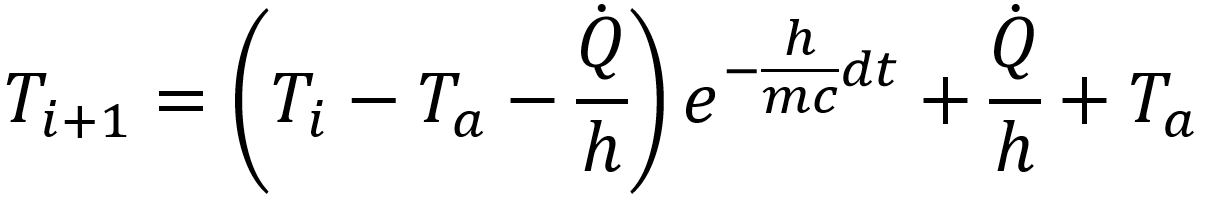
The solution to this differential equation is:
where: |
|
|
|
Ti |
= the current internal temperature of the battery |
|
Ti+1 |
=the temperature after the time dt has elapsed |
This explicit equation is used to model the internal temperature in simulation.
The temperature of the Storage Component can be plotted in the time series results. This is the temperature used to calculate the temperature effects on capacity and the degradation rate.
Temperature Effect on Capacity
Some batteries exhibit variation in capacity with temperature, for example, a decrease in the available energy at cold temperatures. You can enter relative capacity (percent of nominal) versus temperature (Celsius) into the table in the Temperature vs. capacity tab of the Modified Kinetic Battery page in the Library. The Modified Kinetic Battery model fits a quadratic function to the capacity versus temperature data you enter in the table.
In simulation, HOMER effectively adjusts the minimum state of charge up or down based on the current temperature of the battery pack. For example, consider a case where the minimum state of charge specified in the Site Specific Inputs is 20%. At the point in the temperature/capacity curve where the capacity is 100% (often about 20° or 25°C), the minimum state of charge is zero. If, at cold temperatures, the battery capacity is 80% of the nominal value, the minimum state of charge is effectively set to 40%.
It is possible to have a case where the battery is at the minimum state of charge, then the minimum state of charge increases due to a temperature change. If the battery is not charged, the state of charge remains constant, below the minimum state of charge. Of course, the battery is not allowed to discharge any energy until the state of charge is increased to above the minimum state of charge. Likewise, it is possible to exhaust the battery completely. If the battery is warmed and the minimum state of charge decreases accordingly (as in typical capacity versus temperature behavior), HOMER can then take more energy out of the previously exhausted battery.
You must specify a maximum and minimum operating temperature. If the battery temperature is outside of these bounds, the battery does not operate.
Degradation
The Modified Kinetic Battery model tracks degradation using two variables that increase as the pack degrades over its life. One tracks time and temperature over the pack's lifetime, and the other tracks the wear from cycles, adjusted for depth of discharge. Each of these two quantities represents a fractional degradation, from 0 when the pack is new, to 0.2 at the end of life (for the default of a 20% capacity degradation limit).
Functional degradation is modeled as a gradual decrease in storage capacity and increase in series resistance. The capacity degradation follows the maximum of the two values; whichever variable is higher defines the fractional degradation in capacity. The series resistance is scaled larger by the sum of the two degradation variables. See Neubauer 2014 and Smith and Earleywine 2012 for a description of this approach.
Note: In some cases, the Multi-Year Module is necessary to model degradation effects accurately. You can model degradation effects without the Multi-Year module, but only the first year is simulated. This may be adequate for cases where the battery is degraded and replaced after just one year.
Calendar Degradation
The first degradation variable increases with each time step regardless of whether the storage component is being used or idle. The rate of increase of this variable depends only on temperature, as described in the following relationship:
kt = B*e-d/T
In the equation above, kt is the rate of increase of the time-and-temperature degradation variable. B and d are constants fit to data, and T is the temperature in Kelvin. The constant B is scaled such that the degradation variable goes from zero to 0.2 (or the value of the capacity degradation limit when you clicked the Recalculate button) over the course of one lifetime. With this fit, the input data can theoretically be reproduced in simulation. If the battery is held at constant temperature in a simulation, the time and temperature degradation variable reaches 0.2 (or the capacity degradation limit you set) after the time specified for that temperature. You can enter data in the form of years of shelf life versus temperature in the table in the Temperature vs. lifetime tab of the Modified Kinetic Battery page in the Library.
Cycle Degradation
The second degradation variable tracks the cycle fatigue on the battery. The relationship between cycles to failure and depth of discharge (DOD) is described by the following equation:
1/N = ADβ
In the above equation, N is the number of cycles, D is the depth of discharge (a fractional number between 0 and 1), and A and β
are fitted constants. These constants are fitted to the data you enter in the cycles versus depth of discharge table under the Cycle lifetime tab. The constant A is scaled so that the degradation variable goes from zero to 0.2 (or whatever capacity degradation limit you set when you click the Recalculate button) over the course of a lifetime of cycles. Similar to the lifetime and temperature fit described above, the input data is reproduced in simulation; if you run a model where the battery charges and discharges cyclically at a specific DOD, the battery reaches its end of life at the number of cycles specified for the DOD.
In simulation, the Rainflow Counting algorithm is used to convert the battery state-of-charge time series into discrete cycles, each with a DOD. Using the equation above, the fraction of lifetime degradation for each cycle is calculated and summed to calculate the total degradation as follows:
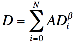
Each cycle has a depth of discharge, Di. The summation is performed over all the cycles calculated using the Rainflow Counting method to calculate the cumulative amount of degradation of the of the cycle-life degradation variable. See ASTM E1049-85(2011)e1 and Manwell, McGowan et. al. 2005 for implementation and justification of the Rainflow Counting algorithm.
Note: Because the temperature effect on battery capacity modifies the minimum state of charge of the battery to change the battery capacity, the number of charge/discharge cycles before the battery's end of life can differ slightly from the specified value. For example, for a battery with a minimum state of charge of 20%, 1,000 cycles to failure at 80% DOD, and capacity that decreases at low temperatures, the minimum state of charge might rise to 25% to model the reduced capacity at lower temperature. In that case, the battery might last more than 1,000 full cycles.
End of Life
The battery is considered dead and is instantly replaced at the "end of life," as determined by the calendar and cycle degradations. The parameters for these two degradation models determine how quickly the battery reaches the end of life. In addition, the "Calculate end of life by:" parameter also affects the end of life calculation. If you select "Sum of calendar and cycling degradation," the battery replacement occurs when the sum of the two degradation values reaches the fraction specified by the Degradation Limit input. If you select "Calendar or cycling degradation, whichever is greater," the battery is replaced when either the time-and-temperature degradation variable or the cycle degradation variable equals the degradation limit (whichever happens first).
The "Sum of calendar and cycling degradation" end-of-life calculation generally produces shorter lifetime and replacement intervals than the "Calendar or cycling degradation, whichever is greater" option. In the modified kinetic model, the sum of the two degradation values corresponds to the relative increase in the series resistance, while the greater of the cycle or calendar degradation values reflects the modeled degradation in battery capacity. So, we can also say that for the first option, the battery end of life occurs when the series resistance increases by the degradation limit (i.e., 20%). For the second option, the battery end of life occurs when the battery capacity decreases by the degradation limit. The best option depends on the specific battery you are modeling and the application.
The Capacity degradation limit sets the percent of degradation at which the battery is replaced. There are two contexts in which you can set the Capacity degradation Limit: in the Library, when you are creating a new battery with the Modified Kinetic Battery model, and in the design view site-specific inputs when you are creating a HOMER model.
When you enter data and calculate parameters in the Temperature vs. lifetime and Cycle lifetime tabs, HOMER takes into account the Capacity degradation limit you have set in the Defaults tab when calculating the fitted constants. This has the result of replicating the data you input in a simulation when the default Capacity degradation limit is used. If you change the Capacity degradation limit in the Defaults tab, you might want to go back to the Cycle lifetime and Lifetime vs. Temperature tabs and Recalculate.
If you change the Capacity degradation Limit under Design, the effect is as you would expect. Increasing the Capacity degradation limit increases the time between battery replacements. You can set a sensitivity for this variable to compare the trade-offs between replacing the storage component sooner and keeping it longer with degraded performance.
See also
