
HOMER Pro 3.16

Wind speed time-series data typically exhibit autocorrelation, which can be defined as the degree of dependence on preceding values. The effect of autocorrelation is shown in Figure 1 below. In the absence of autocorrelation, each data point is completely independent of the previous values and the data points jump up and down at random, as shown in part a) of Figure 1. In a strongly autocorrelated time series, the value in any one time step is strongly influenced by the values in previous time steps, so long periods of high or low values emerge, as shown in part c) of Figure 1. Note that each data set in Figure 1 has the same average and the same Weibull k value. The degree of autocorrelation is the only distinction between the data sets.
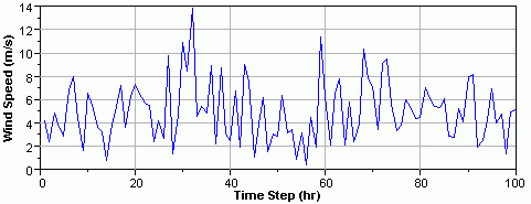
a) Synthetic wind speed time series with no autocorrelation (r1 = 0.0)
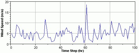
b) Synthetic wind speed time series with moderate autocorrelation (r1 = 0.5)
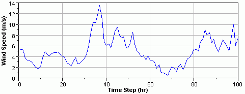
c) Synthetic wind speed time series with strong autocorrelation (r1 = 0.96)
Figure 1: The effect of autocorrelation. All three time series have a mean wind speed of 5 m/s and a Weibull k value of 2.
We know from experience that the wind exhibits autocorrelation. If the wind is blowing strongly at 10 a.m., it is quite likely that it will still be blowing strongly at 11 a.m. But the autocorrelation characteristics of the wind vary from place to place. Before we can explore this any further, we need to learn some fundamentals of autocorrelation.
For a time series z1, z2, z3, ..., zn, we can define an autocorrelation coefficient rk as follows:
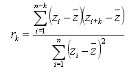
The value rk is the autocorrelation between any two time series values separated by a "lag" of k time units. For a particular time series, we can measure rk for several values of k. The resulting function is known as the autocorrelation function. By definition, r0 = 1.
The autocorrelation function of the wind data measured at Kotzebue, Alaska is shown in Figure 2. This simple autocorrelation function shows that wind speeds at Kotzebue are strongly autocorrelated at short lags and less strongly autocorrelated at longer lags, which is intuitive.
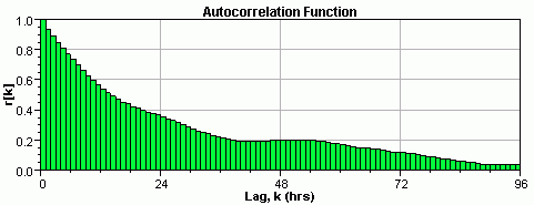
Figure 2: Autocorrelation function for the hourly wind speed data measured at Kotzebue, Alaska.
Kotzebue, however, is an unusual case because there is almost no daily pattern to its wind. A much more common example of a wind speed autocorrelation function is that of San Diego, California, which is shown in Figure 3. The wind speeds at San Diego show a distinct daily pattern, with the afternoons being on average much windier than the mornings. This recurring pattern in the wind speed causes the autocorrelation function to oscillate on a 24-hour period. Because it is usually windy at 3 p.m., the wind speed at 3 p.m. today is strongly autocorrelated with the wind speed at 3 p.m. yesterday and, therefore, with the wind speed at 3 p.m. two days ago, etc.
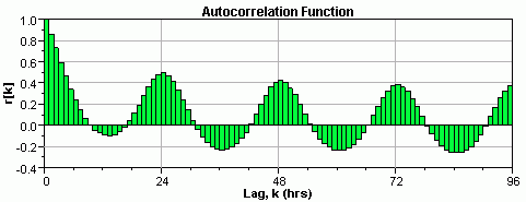
Figure 3: Autocorrelation function for the hourly wind speed data measured at San Diego, California.
HOMER describes the autocorrelation characteristics of wind data with a single number, the autocorrelation factor.
See also
