Mean of Distribution

The simple mean of a set of numbers x₁, x₂, x₃, ..., x_N is given by the following familiar equation:

If you put those numbers into a frequency distribution with m bins, then we could define the mean of that distribution with the following equation:

where:
	y_i	is the midpoint of the i^th bin
	f_i	is the frequency of the i^th bin

This can be called the mean of the distribution. It should be close to the simple mean of the original set of numbers, but it is not guaranteed to be exactly equal.

The distribution contains less information than the original set of numbers, so if all you have is the distribution, you don't know the value of all the numbers that fall within each bin; you only know the frequency of each bin. The best you can do is assume that the values are evenly distributed within each bin. With that assumption, the contribution of each bin to the mean of the distribution is equal to the midpoint of the bin multiplied by the bin frequency. The sum of those products is the mean of the distribution, as the equation above states.

The size of the discrepancy between the mean of the distribution and the simple mean depends on the accuracy of the assumption that the values are evenly distributed within each bin. The discrepancy tends to decrease with decreasing bin size, but not monotonically as the example below shows.

Example

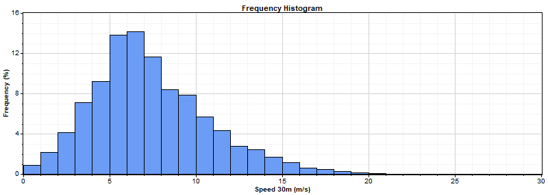
As an example, let's calculate the mean of the following distribution of wind speeds, whose simple mean is 7.4241 m/s:

The following table shows each bin's midpoint, frequency, and the product of midpoint and frequency. The sum of those products gives the mean of the distribution, which we find to be 7.410 m/s:

Bin Endpoints (m/s)		Bin	Occurrences	Frequency	Midpoint
Lower	Upper	Midpoint (m/s)		(%)	x Frequency
0	1	0.5	650	0.912	0.005
1	2	1.5	1,577	2.213	0.033
2	3	2.5	2,965	4.161	0.104
3	4	3.5	5,106	7.166	0.251
4	5	4.5	6,604	9.269	0.417
5	6	5.5	9,862	13.841	0.761
6	7	6.5	10,106	14.184	0.922
7	8	7.5	8,342	11.708	0.878
8	9	8.5	5,990	8.407	0.715
9	10	9.5	5,616	7.882	0.749
10	11	10.5	4,061	5.700	0.599
11	12	11.5	3,102	4.354	0.501
12	13	12.5	2,025	2.842	0.355
13	14	13.5	1,783	2.502	0.338
14	15	14.5	1,227	1.722	0.250
15	16	15.5	863	1.211	0.188
16	17	16.5	475	0.667	0.110
17	18	17.5	381	0.535	0.094
18	19	18.5	220	0.309	0.057
19	20	19.5	143	0.201	0.039
20	21	20.5	69	0.097	0.020
21	22	21.5	41	0.058	0.012
22	23	22.5	26	0.036	0.008
23	24	23.5	11	0.015	0.004
24	25	24.5	5	0.007	0.002
25	26	25.5	1	0.001	0.000
26	27	26.5	0	0.000	0.000
27	28	27.5	0	0.000	0.000
28	29	28.5	0	0.000	0.000
29	30	29.5	0	0.000	0.000
Total			71,251	100	7.410

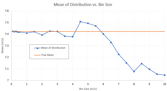
As an experiment, we varied the bin size to see how it affects the discrepancy between the mean of distribution and the simpe mean. Our results confirm that the discrepancy tends to decrease with decreasing bin size, though not monotonically:

As we reduce the bin size in this experiment, the assumption that the numbers are distributed evenly throughout each bin tends to become more accurate. (From the frequency histogram shown above, we can easily see how wrong that assumption is when the bin size is, for example, 5 m/s.) But due to the idiosyncracies of the set of wind speeds on which we base these calculations, that assumption happens to become truer for certain bin sizes than for other nearby bin sizes. The graph above shows that the 1.5 m/s bin size is fortuitous in this way, leading to a more accurate mean-of-distribution value than the 2 m/s or 1 m/s bin sizes. A different original set of numbers would produce a graph with different such zigs and zags, but in general we can expect that smaller bin sizes will result in more accurate values of the mean of the distribution.

Windographer reports the mean of the TAB file distribution on the WAsP page of the Export Data window.